Does the 4% rule survive forward-looking forecasts?

Does the 4% rule still work in 2026?

Key numbers — each row links to the section that carries the full table. Updated 2026-09-27: every figure re-run with the J.P. Morgan correlation matrix actually applied to all six forecasts — see the correction.

Correction (2026-09-27): five forecasts ran without the correlation matrix this page describes

What was wrong. This study says the J.P. Morgan volatilities and correlation matrix were held constant across all six forecasts. The requests behind the 2026-07-10 figures named the correlation source with a misspelled key (correlations_source) that the engine does not read. J.P. Morgan’s own run was unaffected, but BlackRock, Vanguard, GMO, Charles Schwab and Invesco publish no correlation matrix, so those five runs treated US equity, international equity and bonds as independent. J.P. Morgan’s matrix puts the US–international equity correlation at 0.87 and stocks–bonds at 0.30–0.34 (Long-Term Capital Market Assumptions, checked 2026-09-10); ignoring that cut this 45/15/40 portfolio’s annual volatility from about 10.1% to about 7.6%, so those five results overstated the odds of success.

What changed. Every figure on this page was re-run on 2026-09-27 with the key the engine reads, and each run’s own record of which volatilities and correlations it used was checked before it was accepted. The same engine release also compounds the 2.5% inflation rate as an annual rate (previously 2.5%/12 a month, about 2.53% a year), which moves every row by a fraction of a point. 30-year success, pseudo-random paths:

What that does to the conclusions. The headline is stronger, not weaker: no forward-looking forecast comes near the historical near-100%, and three of the five mainstream forecasts now fail in about one path in four or more. The ranking changed — J.P. Morgan, not Charles Schwab, now gives the highest success rate — and the spread in median legacy balance widened from 2.3× to nearly 3×. GMO’s rate moves up three points and it still breaks the rule. The horizon comparison further down was produced by a different request path that already used J.P. Morgan’s matrix, which is why its “stretched” column sat well below the original Result 1; the corrected figures now agree with it to within about half a point. Raw re-run data: research/data/4pct-cme-stress-test-2026-09.json, reproduced by scripts/rerun_4pct_cme_stress_test.py.

The question

William Bengen's 1994 paper (Determining Withdrawal Rates Using Historical Data, Journal of Financial Planning; as published on financialplanningassociation.org, checked 2026-09-10) showed that a 4% inflation-adjusted withdrawal from a 50/50 stock-bond portfolio survived every rolling 30-year window in US history from 1926 to 1976. The "4% rule" became shorthand for safe retirement spending.

That study used historical US returns. Major asset managers — J.P. Morgan, BlackRock, Vanguard, GMO, Charles Schwab, Invesco — now publish forward-looking Capital Market Expectations: their best estimates of returns over the next 7 to 20 years. These forecasts often differ materially from historical averages, especially at current valuation levels.

So the question is concrete: when you swap historical returns for forward-looking expectations, does the 4% rule still hold?

This piece runs the same retirement plan through 10,000 Monte Carlo simulations under each of the six publicly-available forecasts and reports the result.

The plan

One canonical scenario, identical across all six forecasts:

Holding volatility and correlations constant across runs is deliberate: it isolates the effect of each firm's return expectation. Some firms publish their own volatility and correlation estimates; others do not. Using one consistent set lets the comparison be apples-to-apples on the input that varies most across forecasts.

Why the planner can show lower numbers. QuantCalc’s planner defaults to its own historical volatilities, paired with the published correlation matrix. Re-running this same plan with that one change moves the five surviving forecasts from 68.6–85.9% to 65.9–80.8% (same seed, 10,000 pseudo-random paths), and the highest forecast drops from 85.9% to 80.8%. The ranking of the forecasts does not change. The study holds the volatility inputs at one published set so that only the return assumption differs; the sensitivity run is recorded in the page’s source snapshot.

The forecasts

One sentence per source. Each links to its publicly available original. We use only data that has been reported publicly by the firm itself or in widely-circulated financial press; we do not source from paywalled or registration-gated portals.

Of the six, GMO is the outlier — a deliberate one. GMO's framework is mean-reverting: it adjusts current asset prices toward historical fair value over a 7-year horizon. With US large-cap equities trading at elevated cyclically-adjusted earnings multiples (Shiller P/E above 30 in late 2025), GMO's model produces negative real return forecasts for US stocks. The other five firms use building-block approaches that pencil in more modest valuation adjustments.

Result 1: success rate

Probability the portfolio survives 30 years without depletion, by forecast:

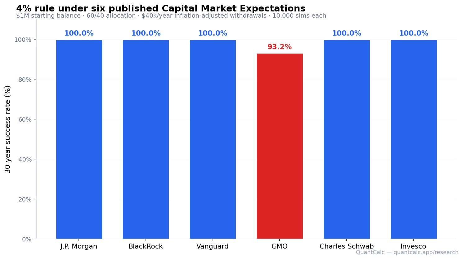
No forecast produces a 100% success rate. The five mainstream forecasts land between 68.6% (Vanguard) and 85.9% (J.P. Morgan); GMO produces 5.6%, meaning 9,439 of 10,000 simulated paths exhausted the portfolio before year 30.

This is the instructive result. The forward-looking forecasts are lower than the long-run historical 1926–2025 averages (~10.2% nominal for US equity), and once the historical tailwind is removed the 4% rule's margin visibly thins: even the strongest forecast here leaves a roughly 1-in-7 chance of depletion over 30 years, and the weakest mainstream forecast nearly a 1-in-3 chance. Why does it still mostly hold?

Because the 4% rule's historical safety margin was wide to begin with. Bengen 1994's 100% historical success rate at 4% on a 50/50 portfolio held with room to spare — but that cushion was built on ~10% nominal US equity returns. Reducing the expected return to the 4.5–6.7% nominal that every forward-looking forecast here pencils in shrinks the margin enough that a 30-year run now carries a real failure probability, 14% to 31%, under all five mainstream forecasts.

GMO breaks rank entirely because its US equity forecast goes negative. A portfolio whose largest single holding has a negative real expected return is a different mathematical object: not a smaller margin, but one that drifts in the wrong direction — and the near-total failure rate reflects it.

Result 2: terminal balance

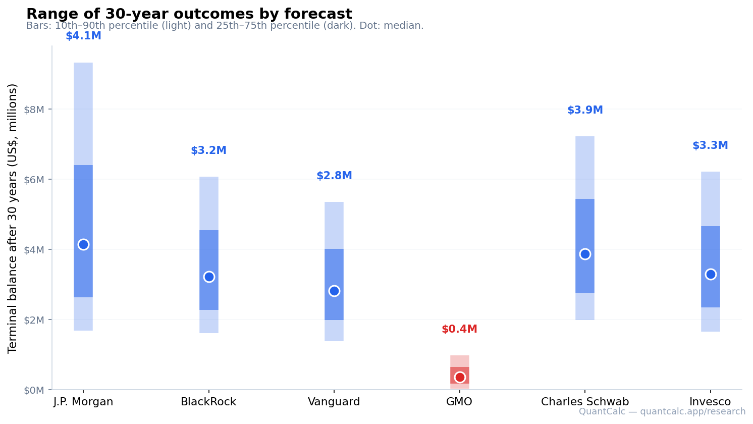
The success-rate chart conceals most of what's interesting. Below: the distribution of terminal balances (after 30 years, in nominal US dollars) under each forecast. The dot is the median; the dark band is the 25th–75th percentile; the light band is the 10th–90th percentile.

The medians:

The headline: even among the five forecasts that keep meaningful survival odds, median terminal balance spans nearly 3× — from $264,366 (Vanguard) to $781,070 (J.P. Morgan) — for an identical plan. Under GMO the median path ends at $0, and every reported percentile through the 95th is $0.

That is a $516,704 difference in median legacy balance between Vanguard and J.P. Morgan for the same plan, the same allocation, the same withdrawal — and it sits on top of survival probabilities that themselves range from 68.6% to 85.9%. Note that the 10th percentile is $0 for all six forecasts: in the worst tenth of outcomes, every one of these forecasts leaves nothing behind.

Why GMO is different

GMO is not pessimistic for its own sake. The firm's framework is explicit and reproducible: forecast US equity returns by reverting current valuations (P/E, Shiller CAPE, dividend yield) to a long-run mean over seven years.

At late-2025 valuation levels — Shiller CAPE above 30, well above the 1926–2024 historical mean near 17, computed from Robert J. Shiller's long-horizon dataset (ie_data.xls, checked 2026-09-10) — that mean-reversion implies several years of below-average price returns. Combined with mediocre starting dividend yields, the model produces a 7-year US equity total return forecast that GMO publishes as a negative real number. After conversion to nominal at a 2.5% inflation assumption, US equity is still roughly −3.5% per year.

For a portfolio that's 45% US equity, that is the difference between marginally building the portfolio and slowly bleeding it. The 4% rule does not survive a sustained negative real return on the largest equity holding, because the inflation-adjusted withdrawal grows at 2.5% per year while the asset shrinks. Sequence-of-returns risk amplifies it.

GMO's model has been historically right and historically wrong. They were notably correct that the late-1990s tech bubble would mean-revert, and notably early — and therefore wrong for years — about the 2010s bull market. We make no claim about whether their current forecast will turn out to be right. The point is that their model produces these numbers, the model is publicly documented, and a 4% retirement plan needs to address what happens if their forecast is correct.

Limitation: five of these six forecasts are not 30-year forecasts

Added 2026-09-16. This study applies each published forecast across the full 30-year horizon. Only J.P. Morgan publishes a 30-year set. GMO publishes seven years; BlackRock, Vanguard and Invesco publish ten; Schwab publishes twenty. Running a seven-year mean-reversion forecast across three decades assumes the reversion never finishes, which is not what its publisher claims.

Re-running the identical plan with each forecast applied over its own published horizon and J.P. Morgan’s 30-year set thereafter (10,000 paths, same allocation, same spending, J.P. Morgan volatility and correlations throughout) shows how much of each result is horizon treatment rather than the forecast itself:

The penalty scales with the stretch. At twenty years it is negligible (0.4 points). At ten years it is material but does not change the conclusion — those forecasts still land well below the historical record. At seven years, applied to an explicitly mean-reverting model, it dominates: the 5–6% figure reported above for GMO is mostly an artefact of the horizon, not a finding about the 4% rule.

The headline conclusion survives: no published forward-looking forecast reproduces the historical near-100% success rate, and the spread between forecasts remains large. But the GMO row should be read as what happens if the next seven years look like GMO’s forecast and nothing reverts afterwards, which is a stronger assumption than GMO makes. Figures re-run on the production engine 2026-09-16 (Sobol QMC paths, before the 2026-09-27 inflation-compounding fix; that fix raised each row by up to about half a point against the Sobol QMC column of that time; the Methodology table’s QMC columns have since been re-run on the engine’s Owen-scrambled sampler).

What this implies for retirees

Three takeaways. None are advice — they're observations from the data.

1. Under forward-looking forecasts, the 4% rule carries real failure risk.

With no other income, none of the six forecasts reproduce the near-100% success rate the historical US record implies. The five mainstream forecasts fail in roughly 1-in-7 to nearly 1-in-3 of 30-year paths. If your prior was that the 4% rule is close to a guarantee, this data says: only against historical returns. Against every published forward-looking forecast, the margin is meaningfully thinner.

2. It breaks entirely if a mean-reverting forecast is right about US equity valuations.

GMO's forecast is the extreme case, at 5.6% success. If you believe equity returns over the next decade will reflect mean reversion from elevated valuations rather than continued historical-average growth, a 4% withdrawal on a 60/40 portfolio is close to a coin flip that lands the wrong way — you would want a materially lower withdrawal rate or a different allocation.

3. Supplemental income and the bequest distribution both change the picture.

This scenario deliberately models a portfolio-only retirement — no Social Security, no pension. Most households have some floor of guaranteed income, which lifts these numbers; the calculator lets you add it. And the legacy distribution is wide: median terminal balance spans nearly 3× across the surviving forecasts, and the 10th-percentile outcome is $0 for all of them. Retirees with bequest motives, or with longer-than-30-year horizons, get more decision-relevant signal from the full distribution than from the headline success rate alone.

Methodology

Engine

QuantCalc's Monte Carlo simulation engine, written in C, with correlated lognormal asset-return modeling via Cholesky decomposition of the published correlation matrix. Withdrawals are inflation-adjusted at a 2.5% deterministic CPI rate, compounded as an annual rate, consistent with the post-1990 anchored inflation regime; further methodology on inflation available. Each simulation runs the full month-by-month portfolio path for 360 months (30 years).

Sampling

Pseudo-random (Mersenne Twister) draws were used as the canonical run rather than the engine's faster default Sobol quasi-Monte Carlo, because QMC is known to converge faster on means but to bias estimates of tail probabilities. The article numbers come from pseudo-random sampling. We re-ran the same scenario under both QMC variants as a robustness check; the comparison appears below.

The success rates are stable across all three sampling regimes; the maximum cross-regime spread is 0.70 percentage points (Invesco, rotated QMC versus pseudo-random). The two QMC columns were re-run on 2026-10-15: since 12 October 2026 the engine Owen-scrambles every Sobol run, which makes its estimates unbiased (methodology), and every QMC figure but one lies inside the pseudo-random run’s own 95% interval (the exception is GMO with the extra rotation, 6.13% against 5.18–6.08%). The pseudo-random run stays the canonical one, so the article’s figures remain comparable with its earlier versions.

Volatility & correlation matrix

Annual volatility per asset class: US equity 15.2%, international equity 18.0%, bonds 5.0%, real estate 15.0%, cash 1.0% (J.P. Morgan published values, from its Long-Term Capital Market Assumptions, checked 2026-09-10). Correlation matrix: J.P. Morgan published values, full 5×5. Held constant across all six return-forecast runs so that only the return assumption varies (true of the figures on this page since the 2026-09-27 re-run; see the correction). The five other firms either don't publish a complete correlation matrix or use modestly different volatility estimates within typical empirical ranges (US equity 15–19%, bonds 5–7%); using one consistent set isolates the return-forecast variable.

Inflation

Deterministic 2.5% CPI applied uniformly to withdrawals across all runs. Stochastic inflation models (AR(1), regime-switching) are available in the QuantCalc engine and produce qualitatively similar conclusions, with slightly higher tail-failure rates under regime-switching. We chose deterministic for this piece to keep the comparison clean and the methodology reproducible by other researchers.

What this analysis does not model

• Guaranteed income floors (Social Security, pensions, annuities). This scenario is deliberately portfolio-only; adding any fixed income raises every success rate above, because less of the $40k/yr need is drawn from the portfolio. The calculator supports these inputs — they are simply not assumed here unless specified.
• Sequence-of-returns risk beyond what i.i.d. monthly returns naturally produce. The engine does not impose macro regimes or autocorrelation.
• Tax drag on withdrawals (no Roth/Traditional/taxable distinction at this layer).
• Healthcare cost shocks, long-term care events, or other lumpy out-of-distribution spending.
• Behavioral changes — actual retirees often dynamically adjust withdrawals in response to portfolio performance.
• Time-varying volatility (GARCH-style), fat-tailed return distributions (Student-t), or regime-shift correlation increases during crises. The QuantCalc engine supports these; this piece does not enable them.

Reproducibility

The full simulation outputs are available below as machine-readable downloads. The re-run is scripted: scripts/rerun_4pct_cme_stress_test.py drives a local QuantCalc engine, refuses any run whose response does not confirm that J.P. Morgan’s volatilities and correlations were used, and writes the files below. With the same engine version and seed the numbers reproduce exactly.

To reproduce in QuantCalc, run a Monte Carlo simulation with these parameters:

{
  "currentAge": 65,
  "retirementAge": 65,
  "endAge": 95,
  "initialSavings": 1000000,
  "monthlyWithdrawal": 3333.33,
  "allocations": [0.45, 0.15, 0.40, 0.0, 0.0],
  "numSimulations": 10000,
  "adjustForInflation": true,
  "inflationRate": 0.025,
  "useQMC": false,
  "seed": 42,
  "cme_source": "vanguard",                  // change per run
  "correlation_source": "jpmorgan",
  "volatility_source": "jpmorgan"
}

Set cme_source to one of: jpmorgan, blackrock, vanguard, gmo, schwab, invesco. The response’s cmeSourcesUsed should read jpmorgan for correlations and volatilities; the resulting successRate and percentiles match the figures in this article.

FAQ

Why use 60/40 instead of Bengen's 50/50?

60/40 is the more common modern reference allocation for retirement and what most contemporary retirement calculators default to. Re-running the analysis at 50/50 (or 70/30) shifts the absolute numbers but not the ranking of forecasts or the qualitative conclusions. The terminal-balance spread tightens slightly at 50/50 because of the lower equity weight, but the GMO outlier persists.

Does the answer change at a 4.5% or 3.5% withdrawal rate?

Yes — and materially. Lowering the withdrawal to 3.5% improves every forecast's odds; raising it to 4.5% worsens them, and GMO remains a near-certain failure at any of these rates. Adding any guaranteed-income floor (Social Security, a pension) improves them further, because less of the annual need is drawn from the portfolio. Because the pseudo-random draws are unseeded, a precise per-rate figure is best generated live — run the withdrawal-rate sweep on your own inputs at quantcalc.app rather than relying on a single quoted number.

Why isn't there a "Historical 1926–2025" comparison?

Because adding it would distract from the main question — how do forward-looking forecasts treat the 4% rule? The historical rolling-window answer is well-known: Bengen-style backtests on actual US return sequences show effectively 100% 30-year survival at 4%. Monte Carlo resampling is a stricter test — it draws returns independently, without the mean reversion embedded in real sequences. For completeness, under the same 60/40 no-other-income plan with QuantCalc's historical 1926–2025 return and volatility inputs, the Monte Carlo success rate is 89.5%, with a median terminal balance of about $1.27M nominal (re-run 2026-09-27 on the current historical inputs; previously 95.9% and $1.45M) — higher than any of the published forward-looking forecasts, but still short of a guarantee once the full withdrawal is drawn from the portfolio.

Found this useful? Run your own retirement plan against multiple forecasts at quantcalc.app. Or read more research: ACA cliff Monte Carlo (2026) · Three problems with the 4% rule · 2026 safe-withdrawal-rate research · Full simulation methodology.

Related research

Two companion Monte Carlo studies that extend the framework above:

• 510,000-path 51-State Retirement Monte Carlo (2026) — the state-tax companion. The same couple in every state: median 30-year income tax and IRMAA from $162,597 to $309,718 (Oregon), success rates from 80.61% to 84.05%. Open dataset, CC-BY-4.0.
• Monte Carlo ACA Cliff 2026: $212k Cost to Early Retirees — what happens to the 4% withdrawal in the pre-Medicare bridge years when the 400% FPL cliff is back. 80,000-path study across four retiree profiles.