Dynamic or static withdrawals: which lasts longer in retirement?
Guardrails cut the 4% rule’s failure rate from 17% to 1.1% — a 94% reduction — by trading depletion for spending cuts, at a 40% legacy cost. Dynamic, by a wide margin — but it pays for that with spending cuts and a smaller legacy. On a 60/40 portfolio over 35 years, the static 4% rule ran out of money on 17% of 10,000 Monte Carlo paths (83.0% plan survival) while paying a flat $40,000 real a year and leaving a median $1.16M legacy; Guyton-Klinger guardrails, starting at $50,000, kept 98.9% of plans solvent (1.1% failure) and spent 15% more over the retirement, at the cost of a 40% smaller median legacy and a real-spending cut in about 22% of years (median worst-case drawdown 27%). The constant-percentage and VPW rules can never run dry, but they cut spending in roughly half of all years. All four rules face the same return paths (common random numbers), in real dollars, pre-tax, single portfolio; engine withdrawal-strategies-1.0.0, published 2026-07-09 — see the strategy table and the allocation sensitivity.
Key numbers — each row links to the section that carries the full table. Updated 2026-09-07; data unchanged (engine withdrawal-strategies-1.0.0).
| Key number | Value | Where on this page |
|---|---|---|
| Plan survival over 35 years, 60/40: static 4% rule vs Guyton-Klinger guardrails | 83.0% vs 98.9% (failure 17% vs 1.1%) | The stability-versus-legacy trade |
| Median lifetime real income: 4% rule vs guardrails | $1,400,000 vs $1,611,103 (+15%) | The stability-versus-legacy trade |
| Median real legacy: 4% rule vs guardrails | $1,161,564 vs $702,640 (−40%) | The stability-versus-legacy trade |
| Guardrails: years with a cut / median worst-case spending drawdown / worst-year income (p10) | 22% / 27% / $21,277 | Downside protection |
| Worst-year income (p10): VPW / constant 5%-of-balance / static 4% rule | $18,549 / $15,134 / $0 | Downside protection |
| Plan survival, 4% rule vs guardrails, at 80/20 and 40/60 | 82.3% vs 97.3%; 80.8% vs 99.5% | Does the allocation change the verdict? |
| Return paths per allocation (shared by all four rules) | 10,000 over 35 years, age 65 to 100, $1,000,000 start | Methodology |
The question
“Dynamic beats static” is easy to say and hard to size. So we ran four withdrawal rules on the identical set of 10,000 Monte Carlo market paths — common random numbers, so every rule faces exactly the same 35-year sequence of returns, and the only thing that differs is the spending rule. The retiree starts at age 65 with $1,000,000, spends for 35 years (to age 100), and everything is measured in real (inflation-adjusted, today’s) dollars. The four rules:
- Static 4% rule. Withdraw 4% of the starting balance ($40,000) and hold that amount constant in real terms every year, regardless of markets. The classic rule from Bengen (1994) and the Trinity study, checked 2026-09-10. It can run out of money.
- Constant 5% of balance. Withdraw 5% of the current balance each year. Income floats with the portfolio; it can never fully deplete, but spending swings hard with the market.
- Guyton-Klinger guardrails. Start at 5%, then adjust with two guardrails on the withdrawal rate (details in Methodology). A dynamic middle path designed to spend more while protecting against ruin.
- Variable Percentage Withdrawal (VPW). Each year withdraw a rising, age-based percentage that amortizes the balance over the years remaining. It deliberately spends the portfolio down toward zero by the end.
The stability-versus-legacy trade, in one table
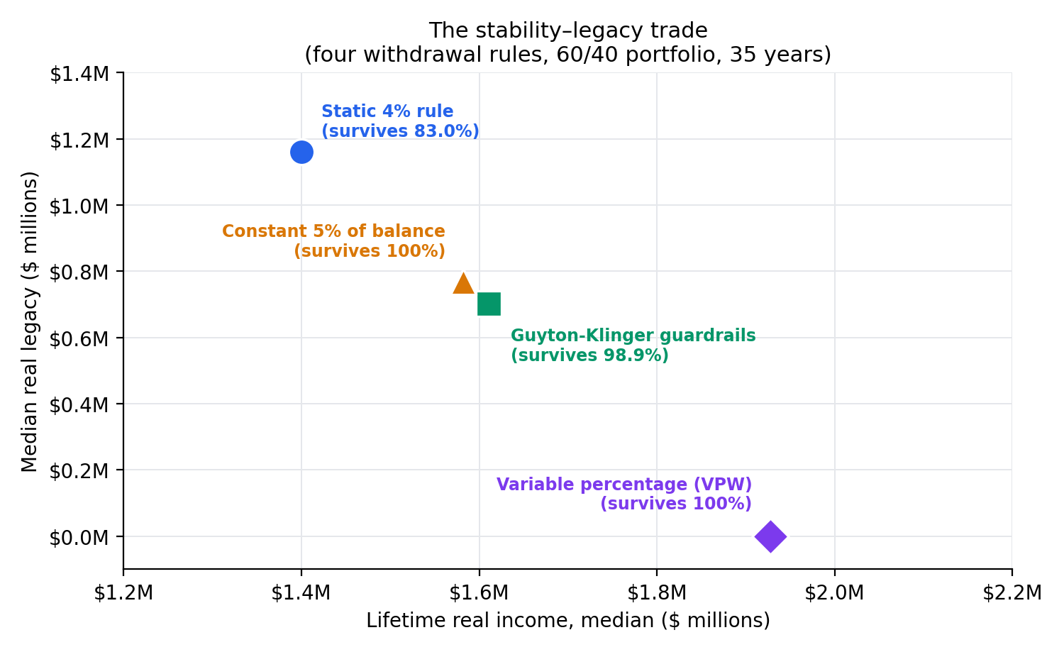
Every number below is for the 60/40 stock/bond portfolio, 10,000 paths, 35 years, real dollars. Plan survival is the share of paths that never failed to fund the intended withdrawal (the constant-percentage and VPW rules scale spending to whatever is there, so they are solvent by construction). “Worst-year income” is the 10th-percentile of each path’s leanest year — the downside a bad-luck retiree actually lives through.
| Strategy | Plan survival (35y) | Starting income | Lifetime income (median) | Worst-year income (p10) | Years with a cut | Max spending drawdown (median) | Median legacy |
|---|---|---|---|---|---|---|---|
| Static 4% rule | 83.0% | $40,000 | $1,400,000 | $0 | 1% | 0% | $1,161,564 |
| Guyton-Klinger guardrails | 98.9% | $50,000 | $1,611,103 | $21,277 | 22% | 27% | $702,640 |
| Constant 5% of balance | 100% | $50,000 | $1,582,068 | $15,134 | 51% | 51% | $769,013 |
| Variable percentage (VPW) | 100% | $56,384 | $1,927,489 | $18,549 | 50% | 50% | $0 |
How to read it. The static 4% rule is the stability-and-legacy champion — a dead-flat $40,000 real every year and a median $1.16M left over — but it also carries the only real failure risk (17%) and, on the paths where it fails, income falls to $0. The dynamic rules almost never leave a retiree penniless, and they spend more over a lifetime, but they demand flexibility: a cut in one year out of five or more, and (for VPW) essentially nothing left at the end.
What the spending actually looks like
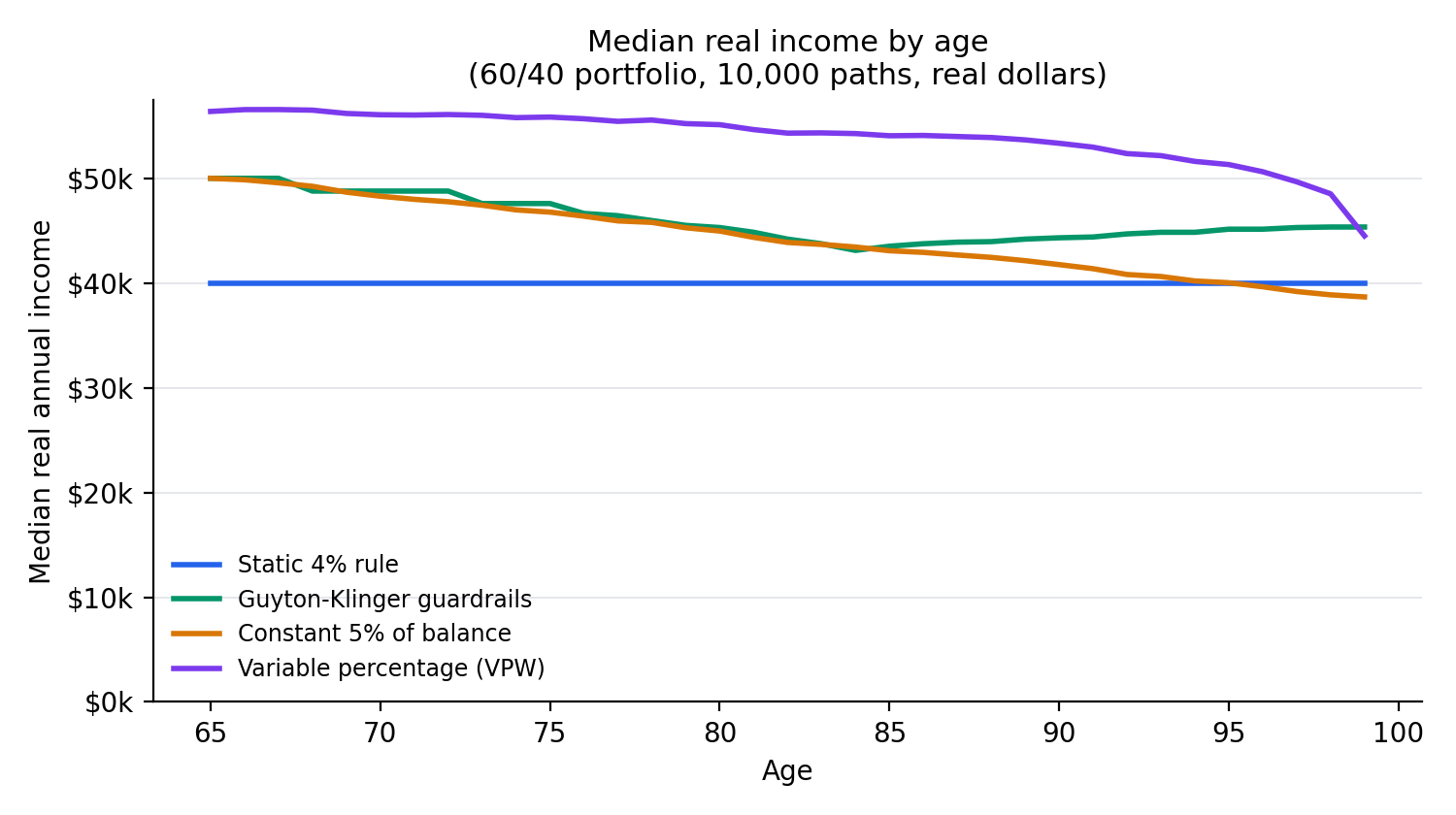
The median real income path makes the personalities plain. The static 4% line is a ruler. The guardrail line starts a quarter higher and stays there with gentle give. The constant-percentage and VPW lines start highest and drift as the portfolio and the amortization schedule dictate.
Downside protection: which dynamic rule cuts most gently?
All three dynamic rules avoid outright ruin, but they are not equal on the downside. In a bad-luck retirement (the 10th-percentile worst year), Guyton-Klinger guardrails leave the most on the table — a worst-year real income of $21,277, versus $18,549 for VPW and $15,134 for the constant-percentage rule. Guardrails also ask for cuts far less often: a cut in about 22% of years, against roughly 51% for the constant-percentage and VPW rules. The static 4% rule, by contrast, asks for a cut in only 1% of years — but that number hides the cliff: when it fails, spending does not taper, it collapses.
Does the allocation change the verdict?
We ran the same four rules on three stock/bond mixes. A bond-heavier portfolio lowers both the failure risk and the legacy of the static 4% rule, but the shape of the trade is unchanged: guardrails eliminate almost all of the 4% rule’s failure rate at every allocation by trading depletion for spending cuts, at the cost of a materially smaller median legacy.
| Allocation | Static 4% rule — plan survival | Guardrails — plan survival | Guardrails median legacy vs. 4% rule |
|---|---|---|---|
| 80/20 | 82.3% | 97.3% | −47% |
| 60/40 | 83.0% | 98.9% | −40% |
| 40/60 | 80.8% | 99.5% | −26% |
What it implies for your withdrawal plan
- The choice is a trade, not a winner. The static 4% rule buys the most predictable spending and the largest legacy, and pays for it with a real (17%) chance of running short. The dynamic rules buy near-certain solvency and higher lifetime spending, and pay for it in spending variability and legacy.
- If flexibility is available, guardrails are the balanced middle. They delivered near-certain plan survival (98.9% — close to the guaranteed solvency of the fraction-of-balance rules), the gentlest downside of the dynamic rules, and 15% more lifetime spending than the 4% rule — as long as you can absorb a cut in roughly 22% of years.
- Match the rule to the money you can flex. If most spending is essential and hard to trim, the variability of a constant-percentage or VPW rule is hard to live with; if much of it is discretionary, the dynamic rules turn that flexibility into higher average spending and a far smaller chance of ruin.
Run your own numbers
Free: enter your own balance, allocation, and spending, and compare static and dynamic withdrawal rules across 10,000 Monte Carlo simulations — success rate, spending, and legacy, side by side. No signup.
Open the Monte Carlo planner →Or read the plain-English comparison guide: Dynamic vs. Static Withdrawal Strategies →
Methodology
Return model. Each year, five asset-class real returns (US equity, international equity, bonds, real estate, cash) are drawn jointly from a multivariate normal built on long-run real capital-market assumptions and a correlation matrix — the same return model used across QuantCalc research (see the sibling ACA subsidy-cliff study). The portfolio’s real return each year is the allocation-weighted sum, and wealth compounds geometrically (the balance is multiplied by one plus that return). The correlation matrix is validated as positive-semidefinite via its Cholesky factor before any paths are drawn. For each allocation, one set of 10,000 return paths is generated and fed to all four strategies (common random numbers), so differences between strategies are differences in the rule, not in luck. The engine is deterministic: two runs produce byte-identical output (seed 20260711).
The withdrawal rules, exactly as implemented.
- Static 4% rule. Year one withdraws 4% of the starting balance; that real amount is held constant thereafter. Bengen (1994); Cooley, Hubbard & Walz (Trinity study, 1998), checked 2026-09-10.
- Constant 5% of balance. Each year withdraws 5% of the current balance — a pure fraction-of-portfolio rule that cannot deplete but tracks the market one-for-one.
- Guyton-Klinger guardrails (Guyton & Klinger, Decision Rules and Maximum Initial Withdrawal Rates, Journal of Financial Planning, March 2006; as published on financialplanningassociation.org, checked 2026-09-10), documented variant: initial withdrawal rate 5%; each year’s inflation raise is applied except it is skipped after a negative nominal-return year when the current withdrawal rate is above the initial rate (the Modified Withdrawal Rule); a Capital Preservation cut of 10% fires when the current withdrawal rate climbs above 1.2× the initial rate (the +20% guardrail), suppressed inside the final 15 years; a Prosperity raise of 10% fires when it falls below 0.8× the initial rate (the −20% guardrail). The portfolio-management (which-sleeve-to-sell) rule is out of scope — a documented simplification.
- Variable Percentage Withdrawal (VPW) (the Bogleheads VPW method): each year withdraws a PMT-style percentage of the current balance that amortizes it over the years remaining to age 100 at the portfolio’s expected real return; the percentage rises with age and the final year withdraws the whole balance, so VPW spends the portfolio down toward zero by design.
Documented assumptions and limitations.
- Real dollars, deterministic inflation. Returns are modeled as real, so spending and balances are real; inflation (2.5%) enters only to reconstruct the nominal return that triggers the Guyton-Klinger inflation-skip rule.
- Single pre-tax portfolio. No Social Security, pension, taxes, fees, asset-location, or glide-path effects; withdrawals are annual (start-of-year), then the remaining balance grows. These can each move the results and are out of scope.
- Normal annual returns. Real returns are drawn from a multivariate normal, which does not capture fat tails or autocorrelation (momentum / mean reversion); a regime-aware companion analysis lives in our Withdrawal Strategy Lab.
- “Success” is solvency, not comfort. A path counts as surviving if it funded every intended withdrawal; for the fraction-of-balance rules that is automatic, so their real story is spending variability, reported here as worst-year income, years-with-a-cut, and maximum spending drawdown.
Reproducibility
The full per-allocation, per-strategy results are published as open data under a CC0 public-domain dedication: results.csv and summary.json. The engine (withdrawal-strategies-1.0.0) is deterministic (seed 20260711): two runs produce byte-identical output. Sources: long-run real capital-market assumptions as used across QuantCalc research (see the ACA subsidy-cliff study and our methodology); Guyton & Klinger, Decision Rules and Maximum Initial Withdrawal Rates (Journal of Financial Planning, 2006); the Bogleheads Variable Percentage Withdrawal method; Bengen (1994) and the Trinity study (Cooley, Hubbard & Walz, 1998) for the 4% rule.
FAQ
Dynamic or static withdrawals: which lasts longer in retirement?
Dynamic, by a wide margin — but it pays for that with spending cuts and a smaller legacy. On a 60/40 portfolio over 35 years, the static 4% rule ran out of money on 17% of 10,000 Monte Carlo paths (83.0% plan survival) while paying a flat $40,000 real a year and leaving a median $1.16M legacy; Guyton-Klinger guardrails, starting at $50,000, kept 98.9% of plans solvent (1.1% failure) and spent 15% more over the retirement, at the cost of a 40% smaller median legacy and a real-spending cut in about 22% of years (median worst-case drawdown 27%). The constant-percentage and VPW rules can never run dry, but they cut spending in roughly half of all years. All four rules face the same return paths (common random numbers), in real dollars, pre-tax, single portfolio; engine withdrawal-strategies-1.0.0, published 2026-07-09 — see the strategy table and the allocation sensitivity.
Do dynamic withdrawal strategies really beat the static 4% rule?
It depends on what you are optimizing. On a 60/40 portfolio over 35 years in this study, the static 4% rule ran out of money on 17% of Monte Carlo paths but paid a perfectly flat real income and left the largest median legacy ($1.16M real). Guyton-Klinger guardrails dropped the failure rate to 1.1% and spent 15% more over the retirement, but left about 40% less legacy and asked for a spending cut in about 22% of years. Dynamic rules win on plan survival and lifetime spending; the static rule wins on predictability and legacy.
How often and how deeply do guardrails cut spending?
In this study, Guyton-Klinger guardrails asked for a real-spending cut in about 22% of years, with a typical (median) worst-case peak-to-trough spending drawdown of 27%. That is gentler than a constant 5%-of-balance rule or VPW, which cut in roughly half of all years. The trade for that flexibility is a much lower chance of depleting the portfolio.
Which withdrawal strategy leaves the most to heirs?
The static 4% rule, by a wide margin: it left a median real ending balance of about $1.16M on a 60/40 portfolio, because it deliberately underspends to stay safe. Guyton-Klinger guardrails left roughly 40% less, and Variable Percentage Withdrawal left essentially nothing — it is designed to spend the portfolio down toward zero by the end of the horizon.
What assumptions does this study use, and can I test my own numbers?
10,000 Monte Carlo paths over 35 years (age 65 to 100), on long-run real capital-market assumptions, with all four rules run on the same return paths (common random numbers). It is a single-portfolio, pre-tax model in real dollars. You can test static and dynamic rules on your own balance, allocation, and spending in the free Monte Carlo planner, which needs no signup; the simulation runs on our servers and your inputs are not stored after the run.
Published 2026-07-09, updated 2026-09-07 by QuantCalc Research. Educational research, not financial advice. Related: dynamic vs. static withdrawal strategies (plain-English comparison guide) · Withdrawal Strategy Lab · sequence-of-returns risk (Monte Carlo).